Note
Click here to download the full example code
Variational coordinate descent for Mixture of Gaussians
How to do Variational Bayes (VB) coordinate descent for GMM.
Here, we train a finite mixture of Gaussians with full covariances.
We’ll consider a mixture model with a symmetric Dirichlet prior:
as well as a standard conjugate prior on the mean and covariances, such that
We will initialize the approximate variational posterior using K=10 randomly chosen examples (‘randexamples’ procedure), and then perform coordinate descent updates (alternating local step and global step) until convergence.
# SPECIFY WHICH PLOT CREATED BY THIS SCRIPT IS THE THUMBNAIL IMAGE
# sphinx_gallery_thumbnail_number = 3

import bnpy
import numpy as np
import os

from matplotlib import pylab
import seaborn as sns

FIG_SIZE = (3, 3)
pylab.rcParams['figure.figsize'] = FIG_SIZE
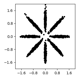
Read bnpy’s built-in “AsteriskK8” dataset from file.
dataset_path = os.path.join(bnpy.DATASET_PATH, 'AsteriskK8')
dataset = bnpy.data.XData.read_npz(
    os.path.join(dataset_path, 'x_dataset.npz'))
Make a simple plot of the raw data
pylab.plot(dataset.X[:, 0], dataset.X[:, 1], 'k.')
pylab.gca().set_xlim([-2, 2])
pylab.gca().set_ylim([-2, 2])
pylab.tight_layout()
Training the model
Let’s do one single run of the VB algorithm.
Using 10 clusters and the ‘randexamples’ initializatio procedure.
trained_model, info_dict = bnpy.run(
    dataset, 'FiniteMixtureModel', 'Gauss', 'VB',
    output_path='/tmp/AsteriskK8/helloworld-K=10/',
    nLap=100,
    sF=0.1, ECovMat='eye',
    K=10,
    initname='randexamples')
Dataset Summary:
X Data
  num examples: 5000
  num dims: 2
Allocation Model:  Finite mixture model. Dir prior param 1.00
Obs. Data  Model:  Gaussian with full covariance.
Obs. Data  Prior:  Gauss-Wishart on mean and covar of each cluster
  E[  mean[k] ] =
   [0. 0.]
  E[ covar[k] ] =
  [[0.1 0. ]
   [0.  0.1]]
Initialization:
  initname = randexamples
  K = 10 (number of clusters)
  seed = 1607680
  elapsed_time: 0.0 sec
Learn Alg: VB | task  1/1 | alg. seed: 1607680 | data order seed: 8541952
task_output_path: /tmp/AsteriskK8/helloworld-K=10/1
        1/100 after      0 sec. |    200.1 MiB | K   10 | loss  6.582634775e-01 |
        2/100 after      0 sec. |    201.3 MiB | K   10 | loss  4.350235353e-01 | Ndiff   68.926
        3/100 after      0 sec. |    201.3 MiB | K   10 | loss  3.454096950e-01 | Ndiff  193.565
        4/100 after      0 sec. |    201.3 MiB | K   10 | loss  3.049230819e-01 | Ndiff  175.237
        5/100 after      0 sec. |    201.3 MiB | K   10 | loss  2.732439109e-01 | Ndiff  108.630
        6/100 after      0 sec. |    201.3 MiB | K   10 | loss  2.326372999e-01 | Ndiff   42.961
        7/100 after      0 sec. |    201.3 MiB | K   10 | loss  2.100254570e-01 | Ndiff    9.814
        8/100 after      0 sec. |    201.3 MiB | K   10 | loss  2.097453779e-01 | Ndiff   10.216
        9/100 after      0 sec. |    201.3 MiB | K   10 | loss  2.094741199e-01 | Ndiff   10.608
       10/100 after      0 sec. |    201.3 MiB | K   10 | loss  2.091535256e-01 | Ndiff   11.009
       11/100 after      0 sec. |    201.3 MiB | K   10 | loss  2.087740779e-01 | Ndiff   11.403
       12/100 after      0 sec. |    201.3 MiB | K   10 | loss  2.083262051e-01 | Ndiff   11.781
       13/100 after      0 sec. |    201.3 MiB | K   10 | loss  2.078022512e-01 | Ndiff   12.135
       14/100 after      0 sec. |    201.3 MiB | K   10 | loss  2.072001819e-01 | Ndiff   12.449
       15/100 after      0 sec. |    201.3 MiB | K   10 | loss  2.065288318e-01 | Ndiff   12.706
       16/100 after      0 sec. |    201.3 MiB | K   10 | loss  2.058118708e-01 | Ndiff   12.883
       17/100 after      0 sec. |    201.3 MiB | K   10 | loss  2.050844132e-01 | Ndiff   12.951
       18/100 after      0 sec. |    201.3 MiB | K   10 | loss  2.043795824e-01 | Ndiff   12.873
       19/100 after      1 sec. |    201.3 MiB | K   10 | loss  2.037146182e-01 | Ndiff   12.598
       20/100 after      1 sec. |    201.3 MiB | K   10 | loss  2.030678434e-01 | Ndiff   12.069
       21/100 after      1 sec. |    201.3 MiB | K   10 | loss  2.022621299e-01 | Ndiff   11.232
       22/100 after      1 sec. |    201.3 MiB | K   10 | loss  2.008648784e-01 | Ndiff   10.057
       23/100 after      1 sec. |    201.3 MiB | K   10 | loss  2.002168334e-01 | Ndiff    8.536
       24/100 after      1 sec. |    201.3 MiB | K   10 | loss  1.995420809e-01 | Ndiff    8.587
       25/100 after      1 sec. |    201.3 MiB | K   10 | loss  1.988594991e-01 | Ndiff    9.312
       26/100 after      1 sec. |    201.3 MiB | K   10 | loss  1.982035545e-01 | Ndiff    9.984
       27/100 after      1 sec. |    201.3 MiB | K   10 | loss  1.974254707e-01 | Ndiff   10.598
       28/100 after      1 sec. |    201.3 MiB | K   10 | loss  1.966834121e-01 | Ndiff   11.131
       29/100 after      1 sec. |    201.3 MiB | K   10 | loss  1.964267444e-01 | Ndiff   11.549
       30/100 after      1 sec. |    201.3 MiB | K   10 | loss  1.961250819e-01 | Ndiff   11.802
       31/100 after      1 sec. |    201.3 MiB | K   10 | loss  1.957730227e-01 | Ndiff   11.830
       32/100 after      1 sec. |    201.3 MiB | K   10 | loss  1.953666781e-01 | Ndiff   11.565
       33/100 after      1 sec. |    201.3 MiB | K   10 | loss  1.949058031e-01 | Ndiff   10.930
       34/100 after      1 sec. |    201.3 MiB | K   10 | loss  1.943977009e-01 | Ndiff    9.860
       35/100 after      1 sec. |    201.3 MiB | K   10 | loss  1.938623040e-01 | Ndiff    8.334
       36/100 after      1 sec. |    201.3 MiB | K   10 | loss  1.933345511e-01 | Ndiff    6.449
       37/100 after      1 sec. |    201.3 MiB | K   10 | loss  1.928570776e-01 | Ndiff    4.458
       38/100 after      1 sec. |    201.3 MiB | K   10 | loss  1.924667495e-01 | Ndiff    2.727
       39/100 after      1 sec. |    201.3 MiB | K   10 | loss  1.921899371e-01 | Ndiff    1.530
       40/100 after      1 sec. |    201.3 MiB | K   10 | loss  1.919922352e-01 | Ndiff    0.873
       41/100 after      1 sec. |    201.3 MiB | K   10 | loss  1.916267958e-01 | Ndiff    0.492
       42/100 after      1 sec. |    201.3 MiB | K   10 | loss  1.909787395e-01 | Ndiff    0.045
... done. converged.
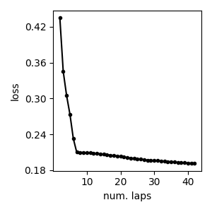
Loss function trace plot
We can plot the value of the loss function over iterations, starting after the first full pass over the dataset (first lap).
As expected, we see monotonic decrease in the loss function’s score after every subsequent iteration.
Remember that the VB algorithm for GMMs is guaranteed to decrease this loss function after every step.
pylab.plot(info_dict['lap_history'][1:], info_dict['loss_history'][1:], 'k.-')
pylab.xlabel('num. laps')
pylab.ylabel('loss')
pylab.tight_layout()
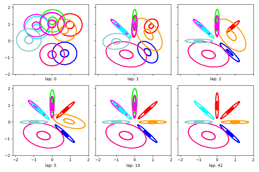
Visualization of learned clusters
Here’s a short function to show the learned clusters over time.
def show_clusters_over_time(
        task_output_path=None,
        query_laps=[0, 1, 2, 5, 10, None],
        nrows=2):
    ''' Read model snapshots from provided folder and make visualizations

    Post Condition
    --------------
    New matplotlib plot with some nice pictures.
    '''
    ncols = int(np.ceil(len(query_laps) // float(nrows)))
    fig_handle, ax_handle_list = pylab.subplots(
        figsize=(FIG_SIZE[0] * ncols, FIG_SIZE[1] * nrows),
        nrows=nrows, ncols=ncols, sharex=True, sharey=True)
    for plot_id, lap_val in enumerate(query_laps):
        cur_model, lap_val = bnpy.load_model_at_lap(task_output_path, lap_val)
        # Plot the current model
        cur_ax_handle = ax_handle_list.flatten()[plot_id]
        bnpy.viz.PlotComps.plotCompsFromHModel(
            cur_model, Data=dataset, ax_handle=cur_ax_handle)
        cur_ax_handle.set_xticks([-2, -1, 0, 1, 2])
        cur_ax_handle.set_yticks([-2, -1, 0, 1, 2])
        cur_ax_handle.set_xlabel("lap: %d" % lap_val)
    pylab.tight_layout()
Show the estimated clusters over time
show_clusters_over_time(info_dict['task_output_path'])
SKIPPED 3 comps with size below 0.00
Total running time of the script: ( 0 minutes 1.888 seconds)