Visualizing learned state sequences and transition probabilities¶

Train a sticky HMM model with auto-regressive Gaussian likelihoods on small motion capture data. Discover how the likelihood hyperparameters might impact performance.

# sphinx_gallery_thumbnail_number = 3

import bnpy
import numpy as np
import os

import matplotlib
from matplotlib import pylab
import seaborn as sns

np.set_printoptions(suppress=1, precision=3)

FIG_SIZE = (10, 5)
pylab.rcParams['figure.figsize'] = FIG_SIZE

Load dataset from file

dataset_path = os.path.join(bnpy.DATASET_PATH, 'mocap6', 'dataset.npz')

dataset = bnpy.data.GroupXData.read_npz(dataset_path)
dataset_biasfeature = bnpy.data.GroupXData(
    X=dataset.X,
    Xprev=np.hstack([dataset.Xprev, np.ones((dataset.X.shape[0], 1))]),
    doc_range=dataset.doc_range)

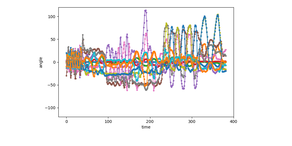
Setup: Function to make a simple plot of the raw data¶

def show_single_sequence(
        seq_id,
        zhat_T=None,
        z_img_cmap=None,
        ylim=[-120, 120],
        K=5,
        left=0.2, bottom=0.2, right=0.8, top=0.95):
    if z_img_cmap is None:
        z_img_cmap = matplotlib.cm.get_cmap('Set1', K)

    if zhat_T is None:
        nrows = 1
    else:
        nrows = 2
    fig_h, ax_handles = pylab.subplots(
        nrows=nrows, ncols=1, sharex=True, sharey=False)
    ax_handles = np.atleast_1d(ax_handles).flatten().tolist()

    start = dataset.doc_range[seq_id]
    stop = dataset.doc_range[seq_id + 1]
    # Extract current sequence
    # as a 2D array : T x D (n_timesteps x n_dims)
    curX_TD = dataset.X[start:stop]
    for dim in range(12):
        ax_handles[0].plot(curX_TD[:, dim], '.-')
    ax_handles[0].set_ylabel('angle')
    ax_handles[0].set_ylim(ylim)
    z_img_height = int(np.ceil(ylim[1] - ylim[0]))
    pylab.subplots_adjust(
        wspace=0.1,
        hspace=0.1,
        left=left, right=right,
        bottom=bottom, top=top)
    if zhat_T is not None:
        img_TD = np.tile(zhat_T, (z_img_height, 1))
        ax_handles[1].imshow(
            img_TD,
            interpolation='nearest',
            vmin=-0.5, vmax=(K-1)+0.5,
            cmap=z_img_cmap)
        ax_handles[1].set_ylim(0, z_img_height)
        ax_handles[1].set_yticks([])

        bbox = ax_handles[1].get_position()
        width = (1.0 - bbox.x1) / 3
        height = bbox.y1 - bbox.y0
        cax = fig_h.add_axes([right + 0.01, bottom, width, height])
        cbax_h = fig_h.colorbar(
            ax_handles[1].images[0], cax=cax, orientation='vertical')
        cbax_h.set_ticks(np.arange(K))
        cbax_h.set_ticklabels(np.arange(K))
        cbax_h.ax.tick_params(labelsize=9)

    ax_handles[-1].set_xlabel('time')
    return ax_handles

Visualization of the first sequence (1 of 6)¶

show_single_sequence(0)

[<AxesSubplot: xlabel='time', ylabel='angle'>]

Setup training: hyperparameters¶

K = 5            # Number of clusters/states

# Allocation model (Standard Bayesian HMM with sticky self-transitions)
transAlpha =   0.5  # trans-level Dirichlet concentration parameter
startAlpha =  10.0  # starting-state Dirichlet concentration parameter
hmmKappa   =  50.0  # set sticky self-transition weight

# Observation model (1st-order Auto-regressive Gaussian)
sF = 1.0          # Set observation model prior so E[covariance] = identity
ECovMat = 'eye'

nTask = 1

Train with EM an HMM with AutoRegGauss observation model¶

Train single model using likelihood without any free parameter

$: x_t ~ mbox{Normal}( A_k x_t-1, Sigma_k)

Take the best of 10 random initializations (in terms of evidence lower bound).

bias0_trained_model, bias0_info_dict = bnpy.run(
    dataset,
    'FiniteHMM', 'AutoRegGauss', 'EM',
    output_path=(
        '/tmp/mocap6/bias0-K=%d-model=HMM+AutoRegGauss-ECovMat=1*eye/'
        % (K)),
    nLap=100, nTask=nTask, convergeThr=0.0001,
    transAlpha=transAlpha, startAlpha=startAlpha, hmmKappa=hmmKappa,
    sF=sF, ECovMat=ECovMat, MMat='eye',
    K=K, initname='randexamples',
    printEvery=25,
    )

Dataset Summary:
GroupXData
  size: 6 units (documents)
  dimension: 12
Allocation Model:  None
Obs. Data  Model:  Auto-Regressive Gaussian with full covariance.
Obs. Data  Prior:  MatrixNormal-Wishart on each mean/prec matrix pair: A, Lam
  E[ A ] =
  [[1. 0.]
   [0. 1.]] ...
  E[ Sigma ] =
  [[1. 0.]
   [0. 1.]] ...
Initialization:
  initname = randexamples
  K = 5 (number of clusters)
  seed = 1607680
  elapsed_time: 0.0 sec
Learn Alg: EM | task  1/1 | alg. seed: 1607680 | data order seed: 8541952
task_output_path: /tmp/mocap6/bias0-K=5-model=HMM+AutoRegGauss-ECovMat=1*eye/1
        1/100 after      0 sec. |    229.7 MiB | K    5 | loss  1.029847757e+10 |
        2/100 after      0 sec. |    229.7 MiB | K    5 | loss  2.401709596e+00 | Ndiff  383.432
       25/100 after      2 sec. |    229.7 MiB | K    5 | loss  2.054112455e+00 | Ndiff    0.371
       50/100 after      4 sec. |    229.7 MiB | K    5 | loss  2.046961483e+00 | Ndiff    5.413
       75/100 after      7 sec. |    229.7 MiB | K    5 | loss  2.021134069e+00 | Ndiff    0.864
      100/100 after      9 sec. |    229.7 MiB | K    5 | loss  2.012157346e+00 | Ndiff    1.147
... done. not converged. max laps thru data exceeded.

Train with EM an HMM with AutoRegGauss observation model¶

Train single model using likelihood WITH free mean parameter

$: x_t ~ mbox{Normal}( A_k x_t-1 + mu_k, Sigma_k)

This is equivalent to including column of all ones into the x-previous, which is how we do it in practice…

Take the best of 10 random initializations (in terms of evidence lower bound).

bias1_trained_model, bias1_info_dict = bnpy.run(
    dataset_biasfeature,
    'FiniteHMM', 'AutoRegGauss', 'EM',
    output_path=(
        '/tmp/mocap6/bias1-K=%d-model=HMM+AutoRegGauss-ECovMat=1*eye/'
        % (K)),
    nLap=100, nTask=nTask, convergeThr=0.0001,
    transAlpha=transAlpha, startAlpha=startAlpha, hmmKappa=hmmKappa,
    sF=sF, ECovMat=ECovMat, MMat='eye',
    K=K, initname='randexamples',
    printEvery=25,
    )

Dataset Summary:
GroupXData
  size: 6 units (documents)
  dimension: 12
Allocation Model:  None
Obs. Data  Model:  Auto-Regressive Gaussian with full covariance.
Obs. Data  Prior:  MatrixNormal-Wishart on each mean/prec matrix pair: A, Lam
  E[ A ] =
  [[1. 0.]
   [0. 1.]] ...
  E[ Sigma ] =
  [[1. 0.]
   [0. 1.]] ...
Initialization:
  initname = randexamples
  K = 5 (number of clusters)
  seed = 1607680
  elapsed_time: 0.0 sec
Learn Alg: EM | task  1/1 | alg. seed: 1607680 | data order seed: 8541952
task_output_path: /tmp/mocap6/bias1-K=5-model=HMM+AutoRegGauss-ECovMat=1*eye/1
        1/100 after      0 sec. |    229.7 MiB | K    5 | loss  1.029794586e+10 |
        2/100 after      0 sec. |    229.7 MiB | K    5 | loss  2.400629439e+00 | Ndiff  352.956
       25/100 after      2 sec. |    229.7 MiB | K    5 | loss  2.022326047e+00 | Ndiff    3.077
       50/100 after      4 sec. |    229.7 MiB | K    5 | loss  2.004862867e+00 | Ndiff    0.832
       75/100 after      7 sec. |    229.7 MiB | K    5 | loss  1.987434495e+00 | Ndiff    0.006
       90/100 after      8 sec. |    229.7 MiB | K    5 | loss  1.987434487e+00 | Ndiff    0.000
... done. converged.

Train with VB an HMM with AutoRegGauss observation model¶

Train single model using likelihood with free mean parameter

$: x_t ~ mbox{Normal}( A_k x_t-1 + mu_k, Sigma_k)

This is equivalent to including column of all ones into the x-previous.

Take the best of 10 random initializations (in terms of evidence lower bound).

bias1vb_trained_model, bias1vb_info_dict = bnpy.run(
    dataset_biasfeature,
    'FiniteHMM', 'AutoRegGauss', 'VB',
    output_path=(
        '/tmp/mocap6/bias1vb-K=%d-model=HMM+AutoRegGauss-ECovMat=1*eye/'
        % (K)),
    nLap=100, nTask=nTask, convergeThr=0.0001,
    transAlpha=transAlpha, startAlpha=startAlpha, hmmKappa=hmmKappa,
    sF=sF, ECovMat=ECovMat, MMat='eye',
    K=K, initname=bias1_info_dict['task_output_path'],
    printEvery=25,
    )


bias0vb_trained_model, bias0vb_info_dict = bnpy.run(
    dataset,
    'FiniteHMM', 'AutoRegGauss', 'VB',
    output_path=(
        '/tmp/mocap6/bias1vb-K=%d-model=HMM+AutoRegGauss-ECovMat=1*eye/'
        % (K)),
    nLap=100, nTask=nTask, convergeThr=0.0001,
    transAlpha=transAlpha, startAlpha=startAlpha, hmmKappa=hmmKappa,
    sF=sF, ECovMat=ECovMat, MMat='eye',
    K=K, initname=bias0_info_dict['task_output_path'],
    printEvery=25,
    )

Dataset Summary:
GroupXData
  size: 6 units (documents)
  dimension: 12
Allocation Model:  None
Obs. Data  Model:  Auto-Regressive Gaussian with full covariance.
Obs. Data  Prior:  MatrixNormal-Wishart on each mean/prec matrix pair: A, Lam
  E[ A ] =
  [[1. 0.]
   [0. 1.]] ...
  E[ Sigma ] =
  [[1. 0.]
   [0. 1.]] ...
Initialization:
  initname = /tmp/mocap6/bias1-K=5-model=HMM+AutoRegGauss-ECovMat=1*eye/1
  K = 5 (number of clusters)
  seed = 1607680
  elapsed_time: 0.1 sec
Learn Alg: VB | task  1/1 | alg. seed: 1607680 | data order seed: 8541952
task_output_path: /tmp/mocap6/bias1vb-K=5-model=HMM+AutoRegGauss-ECovMat=1*eye/1
        1/100 after      0 sec. |    229.7 MiB | K    5 | loss  2.279007765e+00 |
        2/100 after      0 sec. |    229.7 MiB | K    5 | loss  2.278850534e+00 | Ndiff    2.120
       25/100 after      3 sec. |    229.7 MiB | K    5 | loss  2.277292722e+00 | Ndiff    1.431
       50/100 after      6 sec. |    229.7 MiB | K    5 | loss  2.275682910e+00 | Ndiff    0.113
       72/100 after      8 sec. |    229.7 MiB | K    5 | loss  2.275561264e+00 | Ndiff    0.000
... done. converged.
Dataset Summary:
GroupXData
  size: 6 units (documents)
  dimension: 12
Allocation Model:  None
Obs. Data  Model:  Auto-Regressive Gaussian with full covariance.
Obs. Data  Prior:  MatrixNormal-Wishart on each mean/prec matrix pair: A, Lam
  E[ A ] =
  [[1. 0.]
   [0. 1.]] ...
  E[ Sigma ] =
  [[1. 0.]
   [0. 1.]] ...
Initialization:
  initname = /tmp/mocap6/bias0-K=5-model=HMM+AutoRegGauss-ECovMat=1*eye/1
  K = 5 (number of clusters)
  seed = 1607680
  elapsed_time: 0.1 sec
Learn Alg: VB | task  1/1 | alg. seed: 1607680 | data order seed: 8541952
task_output_path: /tmp/mocap6/bias1vb-K=5-model=HMM+AutoRegGauss-ECovMat=1*eye/1
        1/100 after      0 sec. |    229.7 MiB | K    5 | loss  2.274308619e+00 |
        2/100 after      0 sec. |    229.7 MiB | K    5 | loss  2.274112727e+00 | Ndiff    1.193
       25/100 after      3 sec. |    229.7 MiB | K    5 | loss  2.273779830e+00 | Ndiff    0.318
       50/100 after      5 sec. |    229.7 MiB | K    5 | loss  2.273609130e+00 | Ndiff    0.003
       75/100 after      8 sec. |    229.7 MiB | K    5 | loss  2.273609126e+00 | Ndiff    0.001
      100/100 after     11 sec. |    229.7 MiB | K    5 | loss  2.273609125e+00 | Ndiff    0.000
... done. not converged. max laps thru data exceeded.

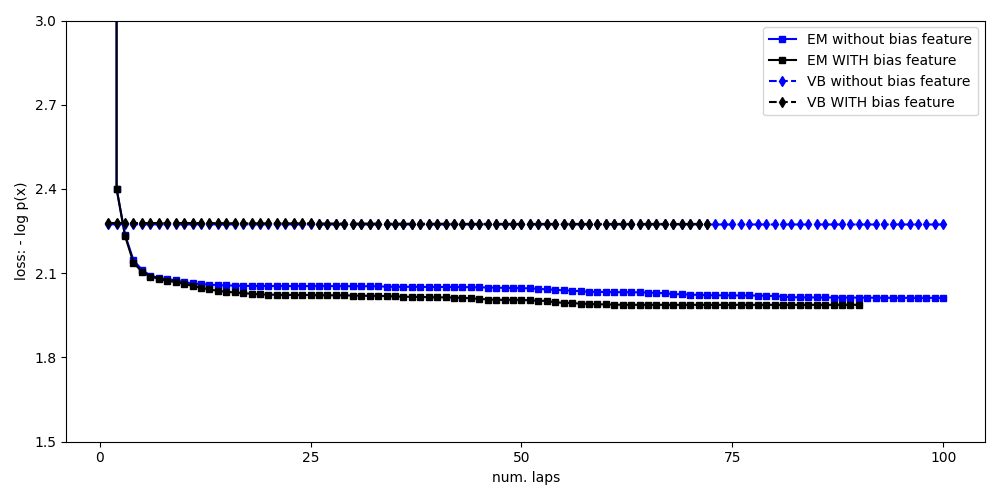
Compare loss function traces for all methods¶

pylab.figure()
markersize = 5
pylab.plot(
    bias0_info_dict['lap_history'],
    bias0_info_dict['loss_history'], 'bs-',
    markersize=markersize,
    label='EM without bias feature')
pylab.plot(
    bias1_info_dict['lap_history'],
    bias1_info_dict['loss_history'], 'ks-',
    markersize=markersize,
    label='EM WITH bias feature')
pylab.plot(
    bias0vb_info_dict['lap_history'],
    bias0vb_info_dict['loss_history'], 'bd--',
    markersize=markersize,
    label='VB without bias feature')
pylab.plot(
    bias1vb_info_dict['lap_history'],
    bias1vb_info_dict['loss_history'], 'kd--',
    markersize=markersize,
    label='VB WITH bias feature')

pylab.legend(loc='upper right')
pylab.ylim([1.5, 3.0])

pylab.xlabel('num. laps')
pylab.ylabel('loss: - log p(x)')
pylab.draw()
pylab.tight_layout()


pylab.show(block=False)

Total running time of the script: ( 0 minutes 36.140 seconds)

Gallery generated by Sphinx-Gallery