Note
Click here to download the full example code
Initialization for Mixtures of Gaussians
How to initialize Gaussian observation models.
We demonstrate a few possible initialization procedures for Gaussian observation models (which include Gauss, DiagGauss, ZeroMeanGauss).
Initialization depends on two key user-specified procedures:
Specifying hyperparameters for the conjugate prior
Specifying how many clusters are created
# SPECIFY WHICH PLOT CREATED BY THIS SCRIPT IS THE THUMBNAIL IMAGE
# sphinx_gallery_thumbnail_number = 2

import bnpy
import numpy as np
import os

from matplotlib import pylab
import seaborn as sns

FIG_SIZE = (3, 3)
SMALL_FIG_SIZE = (2, 2)
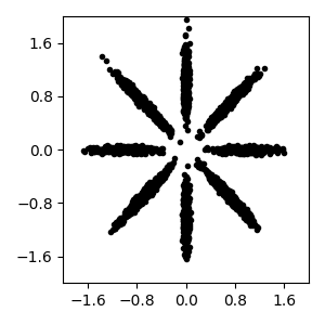
Read bnpy’s built-in “AsteriskK8” dataset from file.
dataset_path = os.path.join(bnpy.DATASET_PATH, 'AsteriskK8')
dataset = bnpy.data.XData.read_npz(
    os.path.join(dataset_path, 'x_dataset.npz'))
Make a simple plot of the raw data
pylab.figure(figsize=FIG_SIZE)
pylab.plot(dataset.X[:, 0], dataset.X[:, 1], 'k.')
pylab.gca().set_xlim([-2, 2])
pylab.gca().set_ylim([-2, 2])
pylab.tight_layout()
Utility function for displaying many random initializations side by side.
def show_many_random_initial_models(
        obsPriorArgsDict,
        initArgsDict,
        nrows=1, ncols=6):
    ''' Create plot of many different random initializations
    '''
    fig_handle, ax_handle_list = pylab.subplots(
        figsize=(SMALL_FIG_SIZE[0] * ncols, SMALL_FIG_SIZE[1] * nrows),
        nrows=nrows, ncols=ncols, sharex=True, sharey=True)
    for trial_id in range(nrows * ncols):
        cur_model = bnpy.make_initialized_model(
            dataset,
            allocModelName='FiniteMixtureModel',
            obsModelName='Gauss',
            algName='VB',
            allocPriorArgsDict=dict(gamma=10.0),
            obsPriorArgsDict=obsPriorArgsDict,
            initArgsDict=initArgsDict,
            seed=int(trial_id),
            )
        # Plot the current model
        cur_ax_handle = ax_handle_list.flatten()[trial_id]
        bnpy.viz.PlotComps.plotCompsFromHModel(
            cur_model, Data=dataset, ax_handle=cur_ax_handle)
        cur_ax_handle.set_xticks([-2, -1, 0, 1, 2])
        cur_ax_handle.set_yticks([-2, -1, 0, 1, 2])
    pylab.tight_layout()
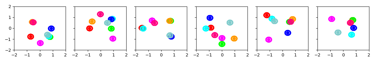
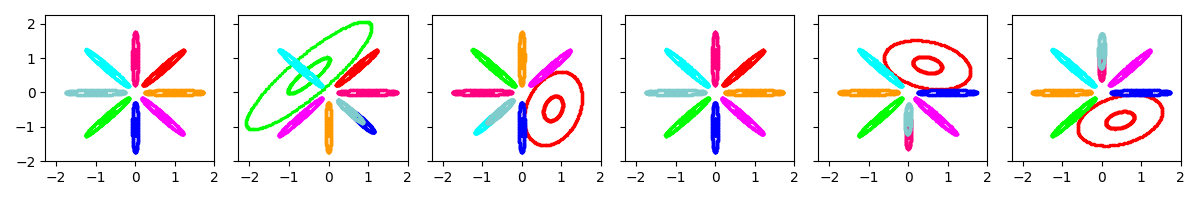
initname: ‘randexamples’
This procedure selects K examples uniformly at random. Each cluster is then initialized from one selected example, using a standard global step update.
Example 1: Initialize with 8 clusters, with prior biased towards small covariances
show_many_random_initial_models(
    dict(sF=0.01, ECovMat='eye'),
    dict(initname='randexamples', K=8))
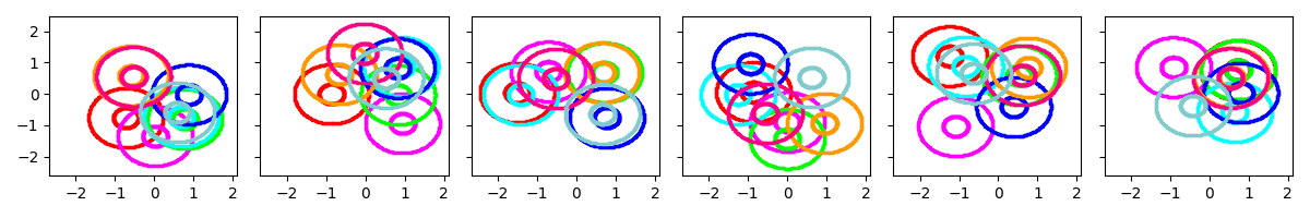
Example 2: Initialize with 8 clusters, with prior biased towards moderate covariances
show_many_random_initial_models(
    dict(sF=0.2, ECovMat='eye'),
    dict(initname='randexamples', K=8))
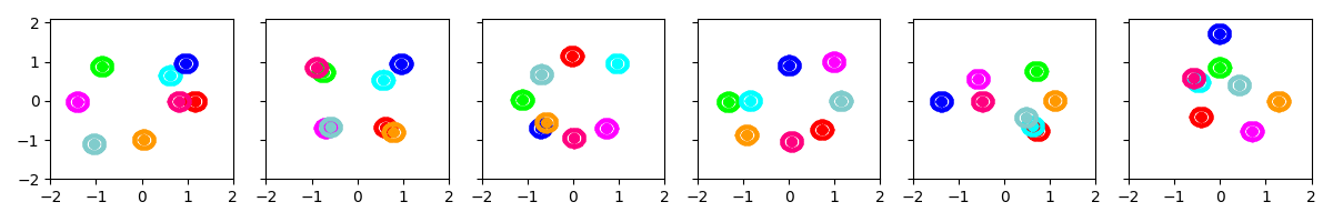
initname: ‘bregmankmeans’
This procedure selects K examples using a distance-biased procedure. First, one example is chosen uniformly at random. Next, each successive example is chosen with probability proportional to the distance from the nearest example in the chosen set.
We measure distance using the appropriate Bregman divergence.
Example 1: Initialize with 8 clusters, with prior biased towards small covariances
show_many_random_initial_models(
    dict(sF=0.01, ECovMat='eye'),
    dict(initname='bregmankmeans', K=8, init_NiterForBregmanKMeans=0))
Example 2: Initialize as above, then allow the k-means algorithm to run for 10 iterations to “refine” the initial clustering.
show_many_random_initial_models(
    dict(sF=0.01, ECovMat='eye'),
    dict(initname='bregmankmeans', K=8, init_NiterForBregmanKMeans=10))
Total running time of the script: ( 0 minutes 3.636 seconds)