Note
Click here to download the full example code
Visualizing learned state sequences and transition probabilities
Train a sticky HDP-HMM model on small motion capture data, then visualize the MAP state sequences under the estimated model parameters by running Viterbi.
Also has some info on how to inspect the learned HMM parameters of a sticky HDP-HMM model trained on small motion capture data.
# sphinx_gallery_thumbnail_number = 3

import bnpy
import numpy as np
import os

import matplotlib
from matplotlib import pylab
import seaborn as sns

np.set_printoptions(suppress=1, precision=3)

FIG_SIZE = (10, 5)
pylab.rcParams['figure.figsize'] = FIG_SIZE
Load dataset from file
dataset_path = os.path.join(bnpy.DATASET_PATH, 'mocap6')
dataset = bnpy.data.GroupXData.read_npz(
    os.path.join(dataset_path, 'dataset.npz'))
Setup: Function to make a simple plot of the raw data
def show_single_sequence(
        seq_id,
        zhat_T=None,
        z_img_cmap=None,
        ylim=[-120, 120],
        K=5,
        left=0.2, bottom=0.2, right=0.8, top=0.95):
    if z_img_cmap is None:
        z_img_cmap = matplotlib.cm.get_cmap('Set1', K)

    if zhat_T is None:
        nrows = 1
    else:
        nrows = 2
    fig_h, ax_handles = pylab.subplots(
        nrows=nrows, ncols=1, sharex=True, sharey=False)
    ax_handles = np.atleast_1d(ax_handles).flatten().tolist()

    start = dataset.doc_range[seq_id]
    stop = dataset.doc_range[seq_id + 1]
    # Extract current sequence
    # as a 2D array : T x D (n_timesteps x n_dims)
    curX_TD = dataset.X[start:stop]
    for dim in range(12):
        ax_handles[0].plot(curX_TD[:, dim], '.-')
    ax_handles[0].set_ylabel('angle')
    ax_handles[0].set_ylim(ylim)
    z_img_height = int(np.ceil(ylim[1] - ylim[0]))
    pylab.subplots_adjust(
        wspace=0.1,
        hspace=0.1,
        left=left, right=right,
        bottom=bottom, top=top)
    if zhat_T is not None:
        img_TD = np.tile(zhat_T, (z_img_height, 1))
        ax_handles[1].imshow(
            img_TD,
            interpolation='nearest',
            vmin=-0.5, vmax=(K-1)+0.5,
            cmap=z_img_cmap)
        ax_handles[1].set_ylim(0, z_img_height)
        ax_handles[1].set_yticks([])

        bbox = ax_handles[1].get_position()
        width = (1.0 - bbox.x1) / 3
        height = bbox.y1 - bbox.y0
        cax = fig_h.add_axes([right + 0.01, bottom, width, height])
        cbax_h = fig_h.colorbar(
            ax_handles[1].images[0], cax=cax, orientation='vertical')
        cbax_h.set_ticks(np.arange(K))
        cbax_h.set_ticklabels(np.arange(K))
        cbax_h.ax.tick_params(labelsize=9)

    ax_handles[-1].set_xlabel('time')
    return ax_handles
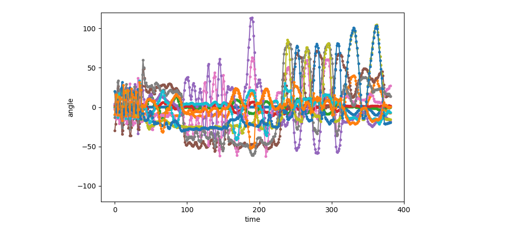
Visualization of the first sequence (1 of 6)
show_single_sequence(0)
[<AxesSubplot: xlabel='time', ylabel='angle'>]
Setup: hyperparameters
K = 5            # Number of clusters/states

# Allocation model (HDP)
gamma      =   5.0  # top-level Dirichlet concentration parameter
transAlpha =   0.5  # trans-level Dirichlet concentration parameter
startAlpha =  10.0  # starting-state Dirichlet concentration parameter
hmmKappa   =  50.0  # set sticky self-transition weight

# Observation model (1st-order Auto-regressive Gaussian)
sF = 1.0          # Set observation model prior so E[covariance] = identity
ECovMat = 'eye'
Train HDP-HMM with AutoRegGauss observation model
Train single model for all 6 sequences.
Do small number of clusters jut to make visualization easy.
Take the best of 5 random initializations (in terms of evidence lower bound).
hdphmm_trained_model, hmmar_info_dict = bnpy.run(
    dataset, 'HDPHMM', 'AutoRegGauss', 'memoVB',
    output_path=(
        '/tmp/mocap6/showcase-K=%d-model=HDPHMM+AutoRegGauss-ECovMat=1*eye/'
        % (K)),
    nLap=100, nTask=5, nBatch=1, convergeThr=0.0001,
    transAlpha=transAlpha, startAlpha=startAlpha, hmmKappa=hmmKappa,
    gamma=gamma,
    sF=sF, ECovMat=ECovMat,
    K=K, initname='randexamples',
    printEvery=25,
    )
Dataset Summary:
GroupXData
  total size: 6 units
  batch size: 6 units
  num. batches: 1
Allocation Model:  None
Obs. Data  Model:  Auto-Regressive Gaussian with full covariance.
Obs. Data  Prior:  MatrixNormal-Wishart on each mean/prec matrix pair: A, Lam
  E[ A ] =
  [[1. 0.]
   [0. 1.]] ...
  E[ Sigma ] =
  [[1. 0.]
   [0. 1.]] ...
Initialization:
  initname = randexamples
  K = 5 (number of clusters)
  seed = 1607680
  elapsed_time: 0.0 sec
Learn Alg: memoVB | task  1/5 | alg. seed: 1607680 | data order seed: 8541952
task_output_path: /tmp/mocap6/showcase-K=5-model=HDPHMM+AutoRegGauss-ECovMat=1*eye/1
    1.000/100 after      0 sec. |    229.7 MiB | K    5 | loss  2.772882295e+00 |
    2.000/100 after      0 sec. |    229.7 MiB | K    5 | loss  2.502603548e+00 | Ndiff  470.393
    3.000/100 after      0 sec. |    229.7 MiB | K    5 | loss  2.426864576e+00 | Ndiff  119.274
   25.000/100 after      3 sec. |    229.7 MiB | K    5 | loss  2.302556401e+00 | Ndiff   18.913
   50.000/100 after      6 sec. |    229.7 MiB | K    5 | loss  2.299789291e+00 | Ndiff    1.326
   75.000/100 after      9 sec. |    229.7 MiB | K    5 | loss  2.285556973e+00 | Ndiff    1.744
  100.000/100 after     12 sec. |    229.7 MiB | K    5 | loss  2.268502057e+00 | Ndiff    1.794
... done. not converged. max laps thru data exceeded.
Learn Alg: memoVB | task  2/5 | alg. seed: 6454144 | data order seed: 7673856
task_output_path: /tmp/mocap6/showcase-K=5-model=HDPHMM+AutoRegGauss-ECovMat=1*eye/2
    1.000/100 after      0 sec. |    229.7 MiB | K    5 | loss  2.789290311e+00 |
    2.000/100 after      0 sec. |    229.7 MiB | K    5 | loss  2.547246672e+00 | Ndiff  332.182
    3.000/100 after      0 sec. |    229.7 MiB | K    5 | loss  2.446687466e+00 | Ndiff   96.506
   25.000/100 after      3 sec. |    229.7 MiB | K    5 | loss  2.282761453e+00 | Ndiff    2.677
   50.000/100 after      6 sec. |    229.7 MiB | K    5 | loss  2.279866842e+00 | Ndiff    0.028
   75.000/100 after      9 sec. |    229.7 MiB | K    5 | loss  2.279866670e+00 | Ndiff    0.003
  100.000/100 after     12 sec. |    229.7 MiB | K    5 | loss  2.279866668e+00 | Ndiff    0.000
... done. not converged. max laps thru data exceeded.
Learn Alg: memoVB | task  3/5 | alg. seed: 6168832 | data order seed: 7360256
task_output_path: /tmp/mocap6/showcase-K=5-model=HDPHMM+AutoRegGauss-ECovMat=1*eye/3
    1.000/100 after      0 sec. |    229.7 MiB | K    5 | loss  2.838795721e+00 |
    2.000/100 after      0 sec. |    229.7 MiB | K    5 | loss  2.614908627e+00 | Ndiff  188.922
    3.000/100 after      0 sec. |    229.7 MiB | K    5 | loss  2.526132362e+00 | Ndiff  143.993
   25.000/100 after      3 sec. |    229.7 MiB | K    5 | loss  2.319895680e+00 | Ndiff    1.371
   50.000/100 after      6 sec. |    229.7 MiB | K    5 | loss  2.318585849e+00 | Ndiff    0.184
   75.000/100 after      9 sec. |    229.7 MiB | K    5 | loss  2.316143371e+00 | Ndiff    0.030
  100.000/100 after     12 sec. |    229.7 MiB | K    5 | loss  2.316143320e+00 | Ndiff    0.001
... done. not converged. max laps thru data exceeded.
Learn Alg: memoVB | task  4/5 | alg. seed: 8205184 | data order seed: 900864
task_output_path: /tmp/mocap6/showcase-K=5-model=HDPHMM+AutoRegGauss-ECovMat=1*eye/4
    1.000/100 after      0 sec. |    229.7 MiB | K    5 | loss  2.805840898e+00 |
    2.000/100 after      0 sec. |    229.7 MiB | K    5 | loss  2.587110039e+00 | Ndiff  428.347
    3.000/100 after      0 sec. |    229.7 MiB | K    5 | loss  2.495055939e+00 | Ndiff  176.781
   25.000/100 after      3 sec. |    229.7 MiB | K    5 | loss  2.338830039e+00 | Ndiff    0.020
   47.000/100 after      6 sec. |    229.7 MiB | K    5 | loss  2.338829969e+00 | Ndiff    0.000
... done. converged.
Learn Alg: memoVB | task  5/5 | alg. seed: 2986368 | data order seed: 6479872
task_output_path: /tmp/mocap6/showcase-K=5-model=HDPHMM+AutoRegGauss-ECovMat=1*eye/5
    1.000/100 after      0 sec. |    229.7 MiB | K    5 | loss  2.828188354e+00 |
    2.000/100 after      0 sec. |    229.7 MiB | K    5 | loss  2.592647224e+00 | Ndiff  435.868
    3.000/100 after      0 sec. |    229.7 MiB | K    5 | loss  2.478529769e+00 | Ndiff  171.138
   25.000/100 after      3 sec. |    229.7 MiB | K    5 | loss  2.302103693e+00 | Ndiff    0.362
   50.000/100 after      6 sec. |    229.7 MiB | K    5 | loss  2.301974529e+00 | Ndiff    0.194
   75.000/100 after      9 sec. |    229.7 MiB | K    5 | loss  2.301969041e+00 | Ndiff    0.000
... done. converged.
Visualize the starting-state probabilities
- start_prob_K1D array, size K
start_prob_K[k] = exp( E[log Pr(start state = k)] )
start_prob_K = hdphmm_trained_model.allocModel.get_init_prob_vector()

print(start_prob_K)
[0.249 0.336 0.032 0.025 0.168]
Visualize the transition probabilities
- trans_prob_KK2D array, K x K
trans_prob_KK[j, k] = exp( E[log Pr(z_t = k | z_t-1 = j)] )
trans_prob_KK = hdphmm_trained_model.allocModel.get_trans_prob_matrix()

print(trans_prob_KK)
[[0.917 0.008 0.052 0.009 0.011]
 [0.025 0.953 0.    0.    0.019]
 [0.09  0.011 0.861 0.035 0.   ]
 [0.012 0.    0.077 0.907 0.   ]
 [0.021 0.026 0.    0.    0.95 ]]
Compute log likelihood of each timestep for sequence 0
- log_lik_TK2D array, T x K
log_lik_TK[t, k] = E[ log Pr( observed data at time t | z_t = k)]
log_lik_seq0_TK = hdphmm_trained_model.obsModel.calcLogSoftEvMatrix_FromPost(
    dataset.make_subset([0])
    )

print(log_lik_seq0_TK[:10, :])
[[ -135.664   -23.757   -42.577  -122.033 -1174.337]
 [ -505.011   -28.26    -52.154  -483.826 -4680.957]
 [  -82.065   -24.821   -45.635   -58.799  -179.048]
 [ -168.085   -28.907   -37.378  -149.684  -678.56 ]
 [ -302.      -28.805   -35.963  -282.073 -2687.59 ]
 [  -70.994   -25.882   -34.915   -68.371  -535.383]
 [ -437.198   -43.6     -50.451  -369.265 -3470.826]
 [  -99.618   -26.81    -51.818   -72.34   -142.138]
 [ -162.653   -32.128   -48.969  -163.484  -942.637]
 [ -582.385   -28.568   -77.439  -573.153 -5090.44 ]]
Run Viterbi algorithm for sequence 0
- zhat_T1D array, size T
MAP state sequence zhat_T[t] = state assigned to timestep t, will be int value in {0, 1, … K-1}
zhat_seq0_T = bnpy.allocmodel.hmm.HMMUtil.runViterbiAlg(
    log_lik_seq0_TK, np.log(start_prob_K), np.log(trans_prob_KK))

print(zhat_seq0_T[:10])
[1 1 1 1 1 1 1 1 1 1]
Visualize the segmentation for sequence 0
show_single_sequence(0, zhat_T=zhat_seq0_T, K=K)
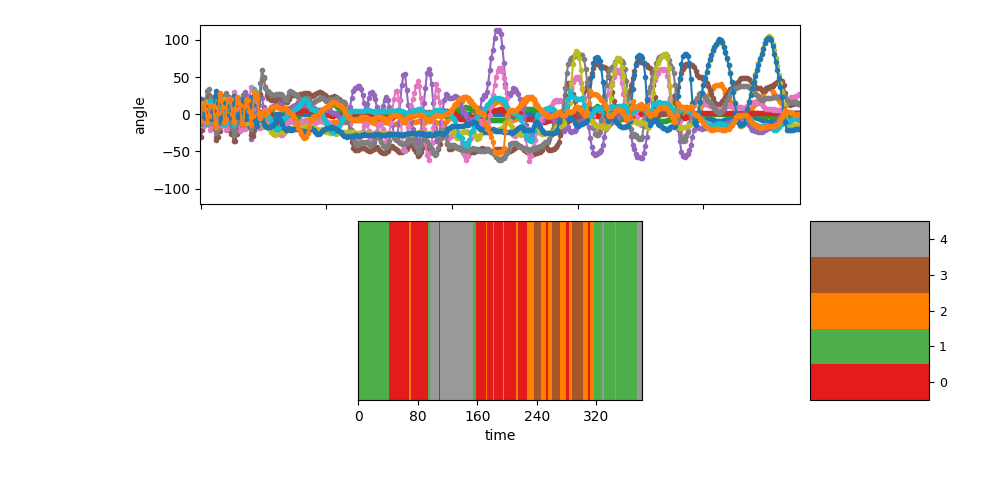
[<AxesSubplot: ylabel='angle'>, <AxesSubplot: xlabel='time'>]
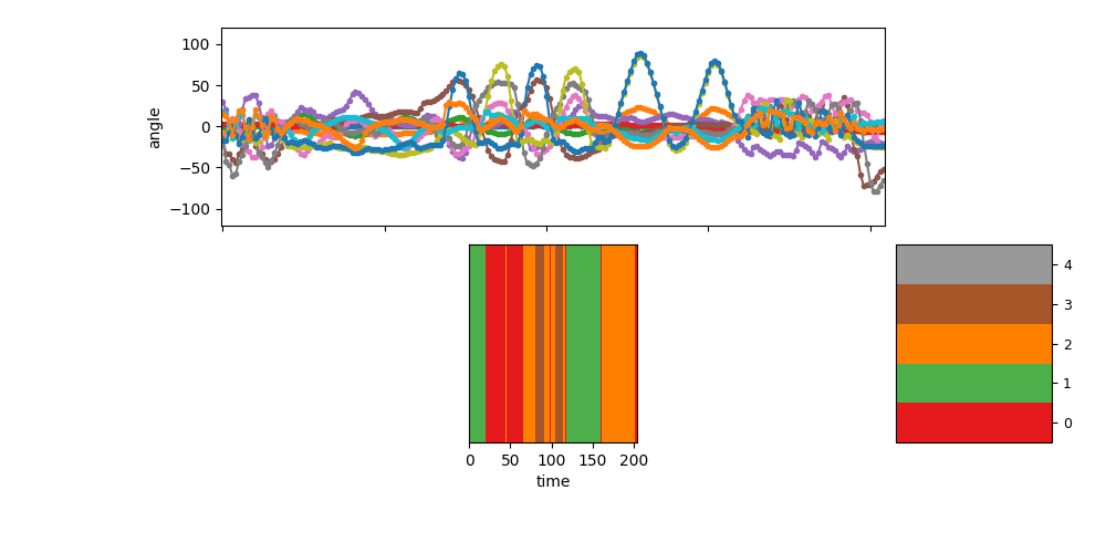
Visualize the segmentation for sequence 1
log_lik_seq1_TK = hdphmm_trained_model.obsModel.calcLogSoftEvMatrix_FromPost(
    dataset.make_subset([1])
    )
zhat_seq1_T = bnpy.allocmodel.hmm.HMMUtil.runViterbiAlg(
    log_lik_seq1_TK, np.log(start_prob_K), np.log(trans_prob_KK))

show_single_sequence(1, zhat_T=zhat_seq1_T, K=K)


pylab.show(block=False)
Total running time of the script: ( 0 minutes 51.747 seconds)